If you've done programming, you’ve likely encountered the big-O notation when analyzing the performance of algorithms. The big-O notation is used to describe how much of a given resource (number of instructions, memory) running an algorithm with given input needs as the size of the input grows.

Popular sorting algorithms like quicksort, mergesort, and heapsort, require, on average, \( O(n \log n) \) comparisons when sorting an array consisting of \( n \) elements. That is to say, as the number of elements in the array grows, the time it takes to sort that array grows slightly — but not a whole lot — faster than in proportion to the size of the array.

But why \( O(n \log n) \), and how come — given the myriads of smart software engineers in the world — nobody has come up with an algorithm that would perform better, say \( O(n \log \log n) \) or even \( O(n) \)?

Turns out that \( O(n \log n) \) is for sure, certainly, definitely the optimal bound. The proof for that is nice and easy to follow after making a few assumptions. After presenting it, I’ll discuss briefly why algorithms like radix sort seem to have lower asymptotic complexity anyway.

What does a computer do when it sorts?

A computer cannot look at an array of keys as a whole and manipulate it globally. Instead, it can:

1. Compare two keys at a time to determine which one of them is larger
2. Manipulate the array somehow (such as swap keys) based on this information
3. Repeat the first two steps some finite number of times until the whole array is sorted

When an algorithm sorts based on comparing keys, it’s called comparison sort. When we talk about needing \( O(n \log n) \) steps to sort an array containing \( n \) keys, we are specifically referring to the number of comparisons.

It’s useful to model a sorting algorithm as a decision tree. At the root of the tree, we have the input array. Each edge of the tree represents a decision the algorithm takes based on the result of a comparison. It takes some route through the decision tree and arrives at the sorted output array at the leaf of the tree.

Let’s demonstrate this with a decision tree describing all the possible paths a bubble sort may take when sorting an array of three keys.

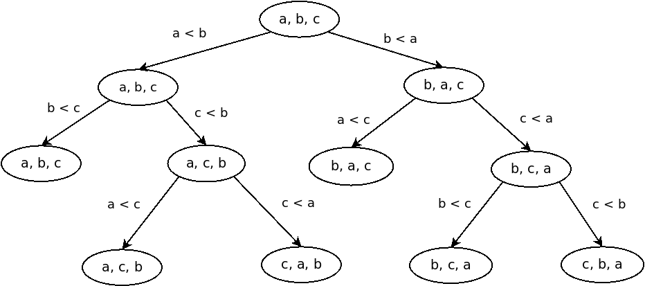
Bubble sort is, rightfully, considered a poor algorithm. It requires \( O(n^2) \) steps — much more than the optimal \( O(n \log n) \) — but it’s easy to follow for demonstration purposes. We see from the picture that sorting three keys completes in three steps, which is as good as it gets for three keys anyway.

The proof of the lower bound

What about a general algorithm for sorting \( n \) keys? To prove that no algorithm can do better than in \( O(n \log n) \) steps in the worst case, it’s not enough to analyze just one particular sorting algorithm. We have to analyze them all.

Let’s start with an arbitrary array of keys \( a, b, ⋯, z \). It is sorted by some decision tree comparing keys pairwise one after another, and arriving at the sorted array at the leaf node, some finite number of steps later. Like this:

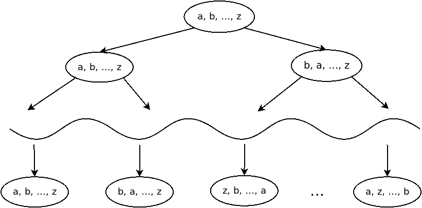
The wavy line represents some arbitrary number of levels between the input and the output.

What can we say about the best possible algorithm sorting this array? Because the input array can potentially be any permutation of the sorted array array, the tree must have at least \( n! \) leaf nodes. Because each comparison only has two possible outcomes, each level of the decision tree has at most twice as many nodes as the previous level. We conclude that

\[ 2^T > n!, \]

where \( T \) is the length of the longest path from the root to a leaf node, i.e. the maximum number of steps it can take to sort an array of \( n \) keys with the algorithm. Because the algorithm is arbitrary, we conclude that no algorithm can beat that bound.

To bring the equation to the more familiar form, we note that \( n! > (½n)^{½n} \), since half of the integers less or equal to \( n \) are greater than \( ½n \). Exploiting this we have

\[ T > \log n! > \log (½n)^{½n} = ½n \log n - ½n, \]

which completes the proof. When talking about the lower bound of running time, as opposed to the upper bound, it is customary to denote the bound as \( Ω(n \log n) \) (using the Greek letter Ω instead of O) when factoring out the uninteresting terms left in the equation.

Radix sort and beating O(n log n)

If you paid attention during your computer science classes, you may have heard of the radix sort algorithm that sorts an array of \( n \) keys having a length of \( b \) bits in \( O(bn) \) steps, thus in a number of steps linear to the size of the array. But we just concluded that it cannot be done better than \( Ω(n \log n) \). What gives?

Remember the assumption that there are at least \( n! \) leaf nodes because there are potentially \( n! \) permutations of the array? This no longer holds when we talk about keys whose size is bounded because there simply isn’t \( n! \) distinct permutations for large enough \( n \). Radix sort indeed exploits the fact that the size of the key is \( b \) bits long, by making \( b \) passes over the array, each time comparing the \( b \mathrm{th} \) bit.

Another way to see it is to imagine we indeed have \( n \) distinct keys of \( b \) bytes each. Then we have \( n ≤ 2^b \), or \( b ≥ \log n \). Comparing this to \( O(bn) \) we have the bound \( O(n \log n) \) once again.